Automobile Analysis
 Photo by CHUTTERSNAP on Unsplash
I created this analysis together with Alexander Kent and Kefan Meng as assessed coursework for one of my Masters’ modules. A big shout out to their invaluable contribution!
The project aim was to investigate the relationship of the MPG (miles per gallon) of a 1980’s car to its other characteristics and question the possibility to use a regression model to reliably predict the MPG.
Update 11/12/21:
This work has been marked on over 87%, with particularly positive feedback on detailed data analysis and creative visualisation methods.
What I have learnt:
- There is no model without first understanding the data.
- Often more information about the raw data is needed for in-depth analysis.
- Model assumptions are vital.
- Multicollinearity is not always the problem - even for highly correlated variables - it depends on what we aim to achieve, understandable model or highly accurate predictions.
- Do not underestimate intuition - fully data-driven analysis can be blinding.
- Report narrative is crucial to aid non-specialist understanding.
1 Explanatory Data Analysis
1.1 Data Preparation
Before we begin the analysis, it is important to address numerous raw data issues. The following steps were taken to prepare the data for modelling:
- In total, there were 18 missing values. To retain possibly important information about indivdual cars that lack only one entry, we imputed the missing values using corresponding medians (we used medians instead of means as the distributions are often skewed). In the case of categorical variables, we imputed a modal value instead.
- To maximise the amount of information the data contains, but address the problem of rare categories, we decided to make intuitive groups (such as
>=fourfor the Cyl variable). Rare observations to which the intuitive categorisation was not possible were removed (5 observations in total: 3 with
4bbl, 1 withmfiand 1 withspfi). For example, there were only three observations with4bbl, and they were almost identical. Moreover, all three contained some missing values, we decided to discard them.EngLoc consists of 202/205 front-located engines. This variable has been discarded since it does not provide any useful information.
After preprocessing, the data consists of 200 observations of 18 variables, of which 5 are categorical (factor), and 13 numerical. Throughout the report we will use italics to distinguish data variables.
1.2 Data Exploration
1.2.1 Categorical Predictors
Let us begin by investigating whether categorical variables reveal any relationship to our main variable of interest - miles per gallon (MPG). Figure 1.1 shows their distribution and corresponding counts. We can see little to no difference between two, and four Doors cars with respect to MPG. Similar can be said for Body, even though there is a slight difference between the types. Drive, Cylinders and Fuel System (FuelSys) seem to have some explanatory power, as the differences between boxes are more apparent. However, we must bear in mind that the majority of occurences are captured by four of less (<=four) cylinders and multi port fuel injection (mpfi) system for Cylinders and FuelSys respectively.
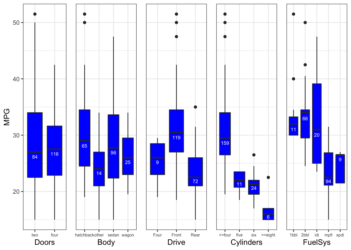
Figure 1.1: Categorical variables
1bbl and 2bbl) tend to have more MPG than cars with multi port fuel injection system (mpfi), which can also be deduced by investigating the last plot of Figure 1 FuelSys boxplot. Moreover, the black line of best fit looks fairly flat when taking into account all points. However, if we split the data into two engine types groups, the relationships are much stronger. In addition to CompRatio, PeakRPM and Stroke are also related to fuel type, with diesel cars generally having less PeakRPM and longer Stroke. It is worth noting that after removing extreme petrol value (11.5), its corresponding \(R^2\) would increase from 0.18 to 0.25, i.e. about 25% of MPG variability could be explained by the CompRatio petrol engine type alone. In the next section we take a closer look at numerical variables and how they interact with MPG.
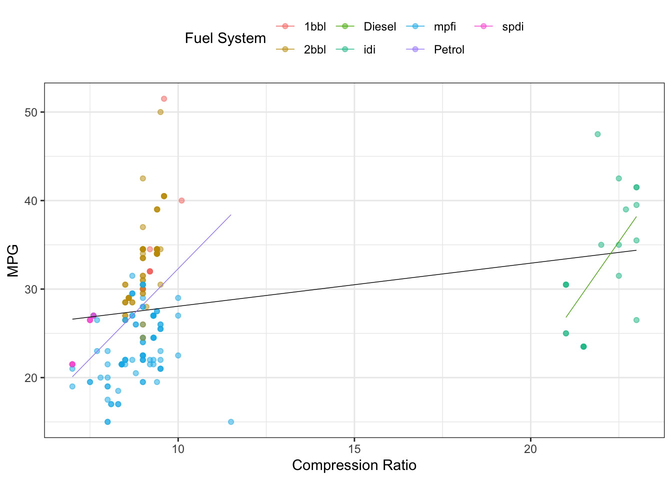
Figure 1.2: Clusters
1.2.2 Correlation
To help us identify the variables’ impact on MPG, we plot the correlation matrix (Figure 1.3). We can immediately notice a triangle with moderate to high correlations between variables. Even at this stage of the analysis we can deduce that the data is highly multicollinear, and we will need to address this problem before modelling. In the next plots, we try to demonstrate why such strong relationships occur. Surprisingly, all numerical predictors but CompRatio are negatively correlated with MPG. By referring back to the brief document, we can understand why, for example, WhlBase is highly correlated with Len - they are very similar measurements.
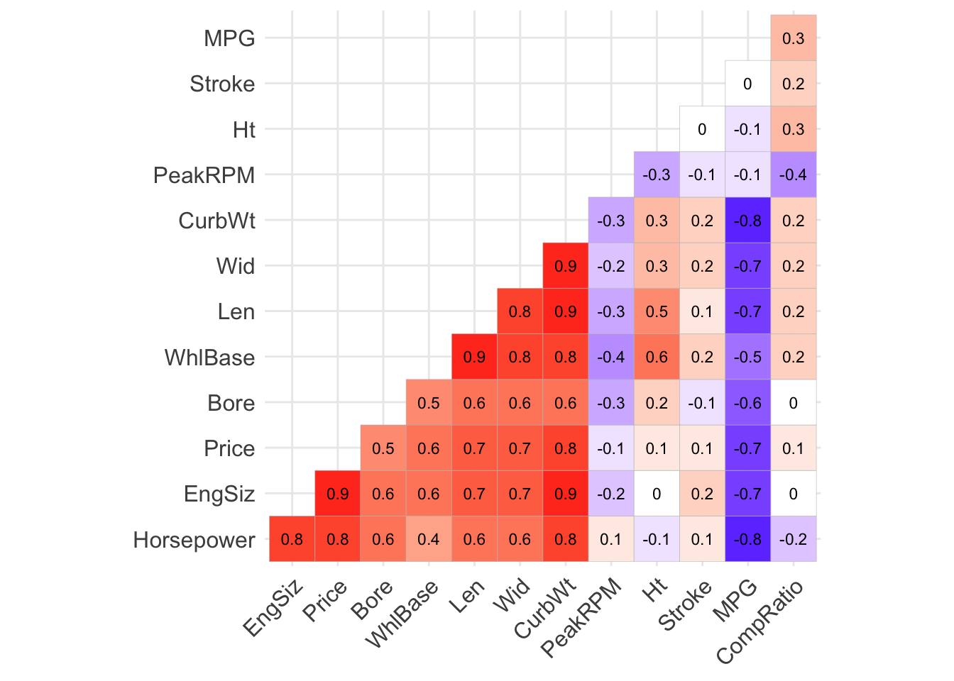
Figure 1.3: Correlations
1.2.3 Horsepower
The correlation bewteen Horsepower and MPG is considerable. Figure 1.3 also shows a correlation of up to 0.8 between Horsepower, EngSize, and CurbWt, We explore how they influence each other in a functional sense. Horsepower is a unit of power, it is highly correlated with EngSiz since larger EngSiz implies more cylinders, and the more cylinders there are, the more petrol is used and more horsepower is generated. Also, the more cylinders there are, of course, the heavier the vehicle will be. Figure 1.6 shows the relation between these variables coloured by the number of cylinders. Cars with more horsepower usually consume more fuel which we can clearly see on the plot. Moreover more cylinders result in more horsepower - the majority of cars have four cylinders (only one car has 3). Moreover, cars with more than four cylinders tend to have a rear drive system, which can be seen on Figure 1.4. We also note an inverse relationship between Horepower and MPG.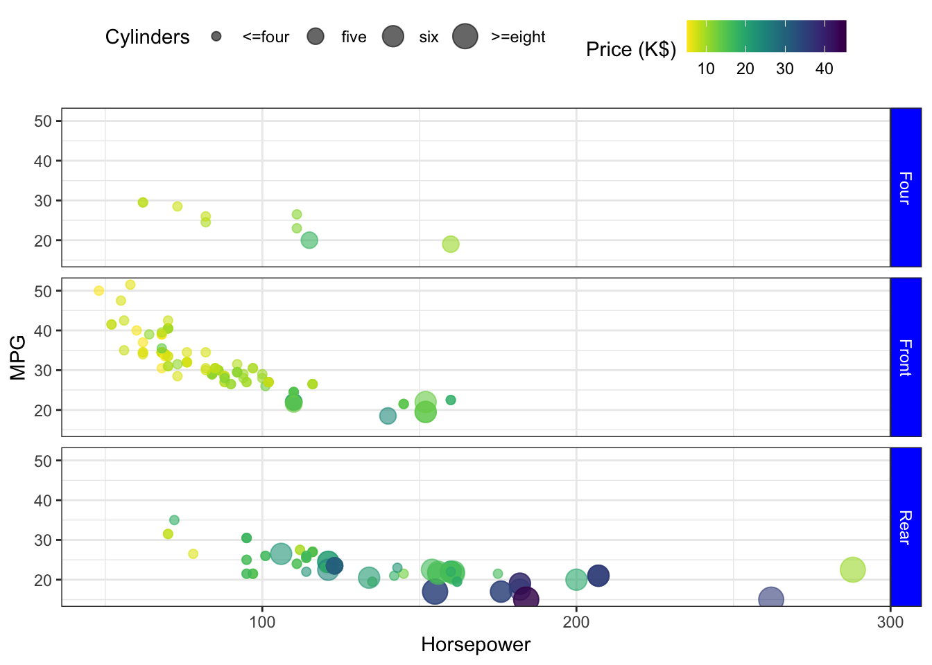
Figure 1.4: Horsepower
1.2.4 Cars Size
A significant number of highly correlated variables constitute cars size or their engine measurements. The bigger the engine, the bigger we expect a car to be. Indeed, Figure 1.5 confirms this presumption. Furthermore, the heavier the engine, the larger it must be, which can be seen on Figure 1.6. Also, the number of cylinders influences the curb weight, and therefore engine size. Even though four cylinders cars dominate, there is an observable pattern for cars with more cylinders - not surprisingly, they tend to increase engine size and weight. When we recall that WhlBase and Len are similar measurements, and Bore measures a diameter of each cylinder, we begin to understand the relation between these variables.
Using only Len, Wid, WhlBase and CurbWt to predict MPG reveals that only CurbWt and WhlBase are influential. This suggests that Len and Wid affect MPG not because of wind resistance or otherwise, but mainly because we need more volume to accommodate more cylinders (more weight) and the larger frame also causes more weight. Our intuition would agree that when the vehicle is heavier, it does more work to travel the same distance and therefore uses more fuel, so we expect Len and Wid to not be important in our model while CurbWt will retain predictive power. Since the correlation between WhlBase and MPG is only 0.5, and it is largely due to correlation with CurbWt, we do not expect to keep this variable either. We will see whether these predictions agree with our model choice during variables selection in the modelling section of this report.
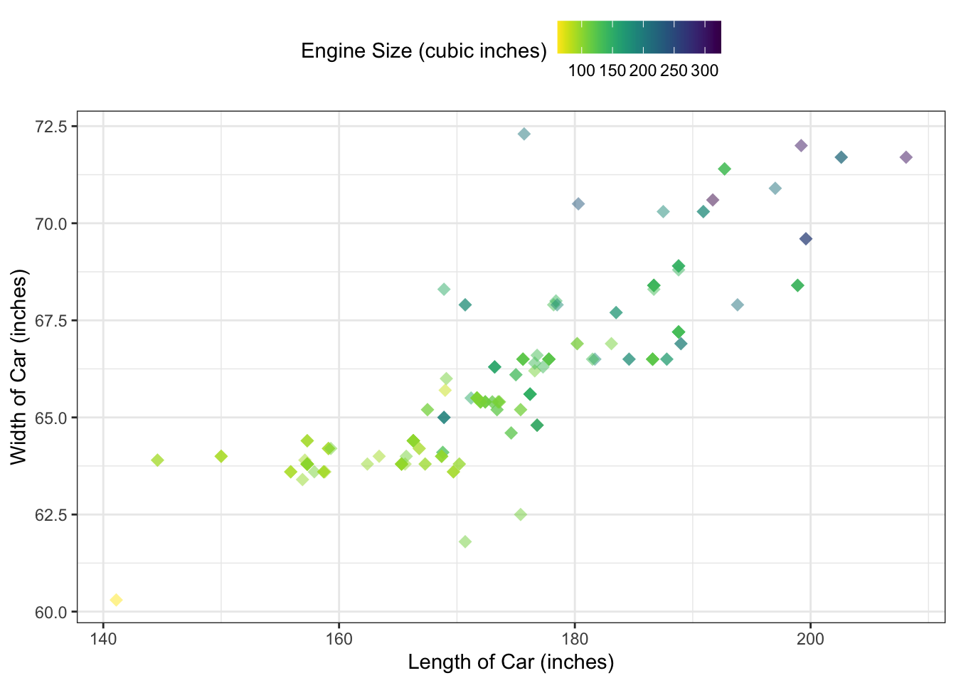
Figure 1.5: Cars size
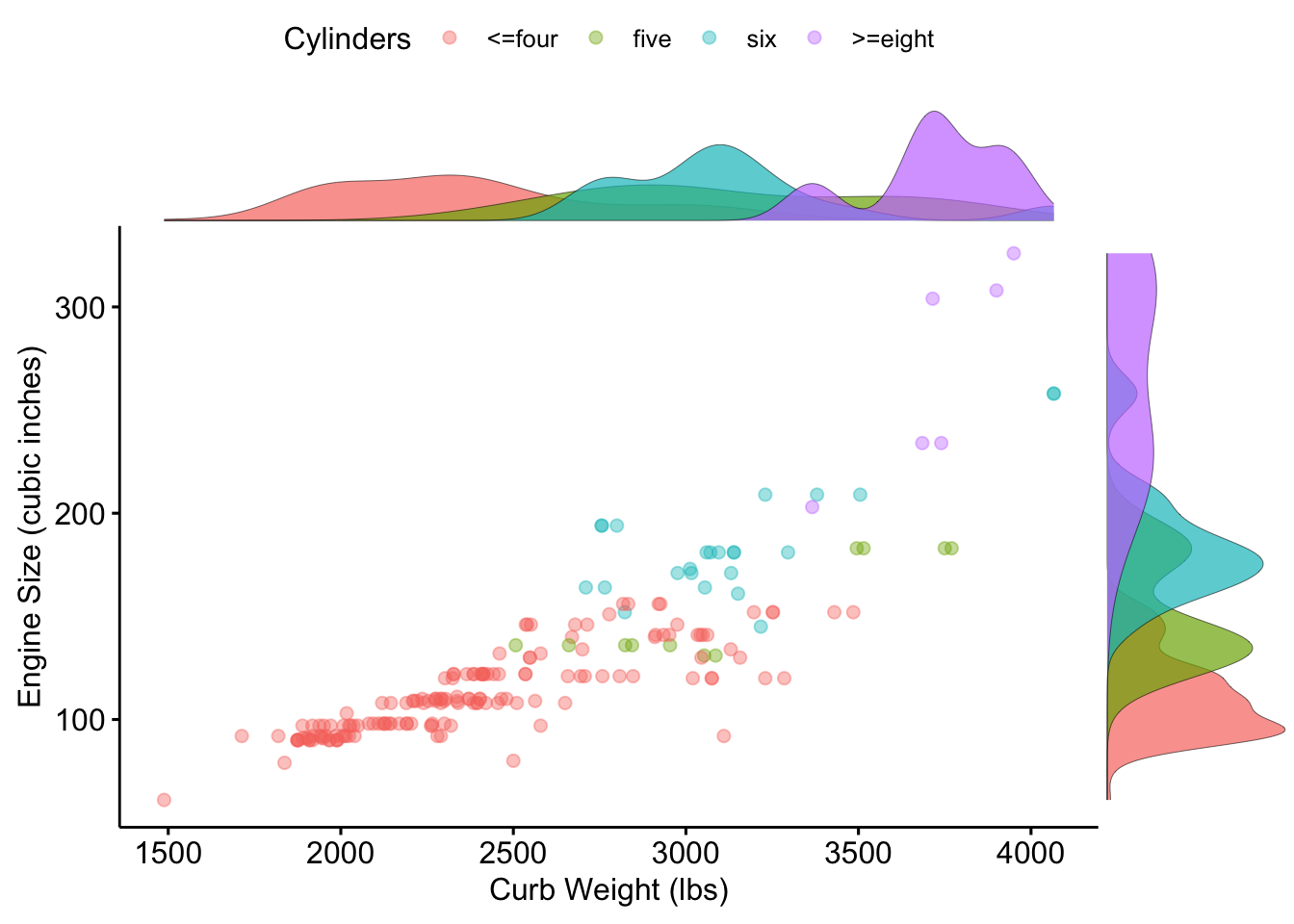
Figure 1.6: Cars engine
1.2.5 Price
The last variable that seem to highly impact MPG is Price. Intuition tell us that it should not be a direct factor when it comes to predicting MPG. However, the high correlation suggests otherwise. Obviously, many other predictors also highly influence Price, for example cars size, engines, or horsepower. The latter being particularly good at predicting Price. Figure 1.4 confirms this belief as we can clearly see that the higher the car costs, the more horsepower it tends to have. However, there is one interesting outlier| MPG | Doors | Body | Drive | WhlBase | Len | Wid | Ht | CurbWt | EngSiz | FuelSys | Bore | Stroke | CompRatio | Horsepower | PeakRPM | Price | Cylinders |
|---|---|---|---|---|---|---|---|---|---|---|---|---|---|---|---|---|---|
| 22.5 | two | hatchback | Rear | 98.4 | 175.7 | 72.3 | 50.5 | 3366 | 203 | mpfi | 3.94 | 3.11 | 10 | 288 | 5750 | 10295 | >=eight |
| MPG | Doors | Body | Drive | WhlBase | Len | Wid | Ht | CurbWt | EngSiz | FuelSys | Bore | Stroke | CompRatio | Horsepower | PeakRPM | Price | Cylinders |
|---|---|---|---|---|---|---|---|---|---|---|---|---|---|---|---|---|---|
| 21 | two | other | Rear | 89.5 | 168.9 | 65 | 51.6 | 2756 | 194 | mpfi | 3.74 | 2.9 | 9.5 | 207 | 5900 | 32528 | six |
| 21 | two | other | Rear | 89.5 | 168.9 | 65 | 51.6 | 2756 | 194 | mpfi | 3.74 | 2.9 | 9.5 | 207 | 5900 | 34028 | six |
It is hard to tell why such duplicates occur, one may speculate that they differed by some other characteristics our data did not record. In total, there were 9 such pairs.
2 Modelling
2.1 Initial Considerations
Following our EDA, and the apparent clusters that formed when considering CompRatio and MPG, we will modify the data and cluster the FuelSys variable into two types: idi (diesel engines) and Other (various petrol engines). We will then include an interaction term in our model which helps us model the effect of belonging to either of these two clusters.
Firstly, let us consider some initial models wherein we will include all variables and inspect the diagnostic plots to see if our modelling assumptions hold and our models are valid. The most simple model will be to fit a model of MPG against all the explanatory variables. As we saw in the EDA section, there appears to be an inverse relationship between the dependent variable and some of the explanatory variables, thus we will also consider a model where we transform some of them by taking their reciprocal. The following table shows the correlation between MPG and untransformed, and transformed explanatory variables respectively.
| WhlBase | Len | Wid | Ht | CurbWt | EngSiz | Bore | Stroke | CompRatio | Horsepower | PeakRPM | Price | |
|---|---|---|---|---|---|---|---|---|---|---|---|---|
| Untransformed | -0.53 | -0.71 | -0.68 | -0.12 | -0.80 | -0.71 | -0.59 | -0.03 | 0.29 | -0.80 | -0.05 | -0.70 |
| Transformed | 0.54 | 0.72 | 0.68 | 0.11 | 0.84 | 0.79 | 0.59 | -0.01 | -0.37 | 0.91 | 0.05 | 0.79 |
We can see from this table that the best candidate variables to transform are EngSiz, CompRatio, Horsepower and Price, as the magnitude of their correlation increases notably after transformation. We fit two models, one with no transformed variables, and one where these four variables are transformed by taking their reciprocal.
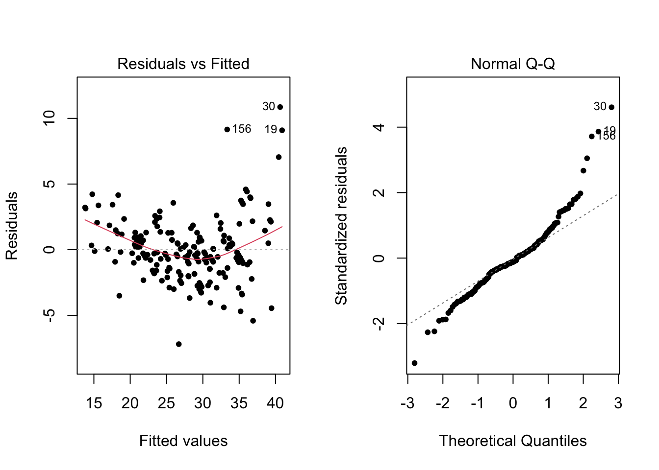
Figure 2.1: Diagnostic plots for model with no transformed explanatory variables
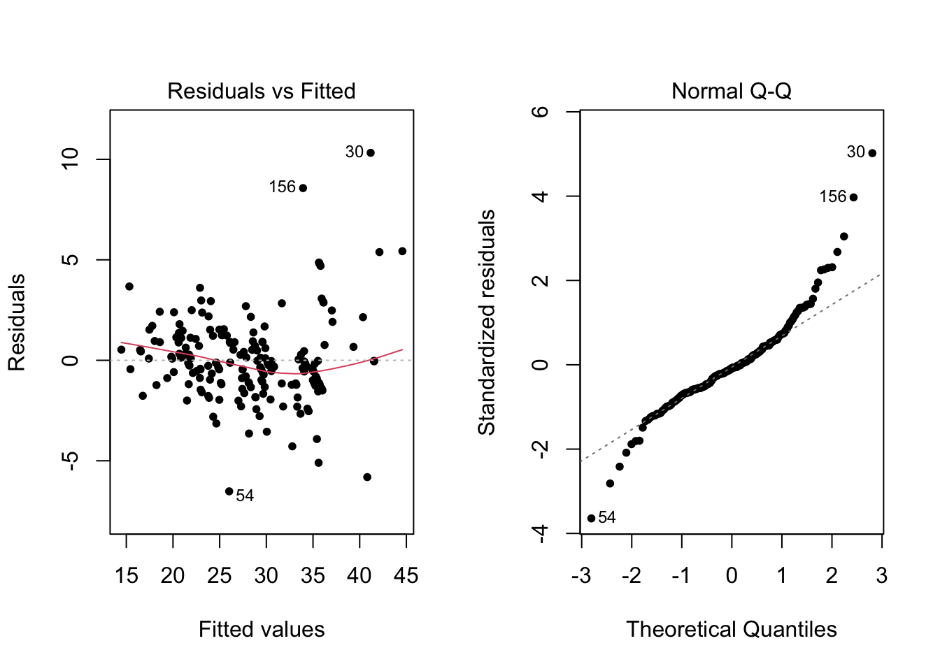
Figure 2.2: Diagnostic plots for model with transformed explanatory variables
| R2 | Adjusted R2 | |
|---|---|---|
| Model 1 | 0.875 | 0.859 |
| Model 2 | 0.904 | 0.892 |
In terms of the \(R^2\), we have high values where at least \(86\%\) of the variance in MPG can be explained by our model. This suggests strong predictive power. The adjusted \(R^2\), which accounts for the fact that more complicated models will perform better, and so penalises such models to encourage simpler models that still predict well, are similarly high. However, in both cases in the residuals plot we observe heteroscedasticity of the errors (that is, the variance of the errors change as the fitted values change), and a noticeable “smile” of the residuals which shows that the mean of residuals is non-zero. Further, the Q-Q plot also shows a large number of observations in the tails that deviate from the expected straight line.
Figure 2.1 and 2.2 suggest that despite the predictive power of our model, there is a violation of our modelling assumptions. This in particular weakens the validity of any statistical inference we carry out as these procedures assume that the modelling assumptions hold. Consequently, our conclusions on what variables are important in determining fuel efficiency may not be correct, limiting the usefulness of our model.
2.2 Transformation of Dependent Variable
As our main issue is the non-normality and heteroscedasticity of the errors which is not resolved by transforming the independent variables, we will now instead consider transforming our dependent variable: MPG. To find the optimal transformation, we will use what is called a “boxcox” transformation, where we aim to transform \(y\) to \(y^\lambda\) (or \(\textrm{log}(y)\) in the case \(\lambda=0\)).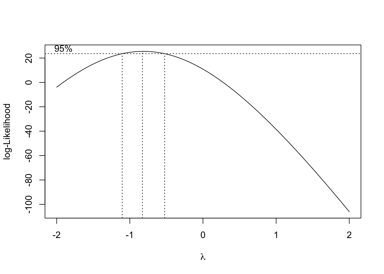
Figure 2.3: Profile likelihood for boxcox transformation
Using the boxcox function, we find that the optimal value of \(\lambda\) for the transformation is approximately \(-\frac{9}{10}\) (the \(\lambda\) where the height of the curve is maximised), which corresponds to transforming \(y=MPG\) into \(y_{transformed}=MPG^{-\frac{9}{10}}\). However, the \(95\%\) confidence interval for this \(\lambda\) is approximately \([-1.1,-0.5]\) and as \(-1\) lies in this confidence interval, which corresponds to the simpler transformation \(y_{transformed}=\frac{1}{MPG}\), we shall use \(\lambda=-1\) instead. This transforms our MPG variable into a variable giving the number of gallons needed on average to traverse one mile, which we shall refer to as Gallons per Mile (GPM).
2.2.1 Model Diagnositcs
We now fit a model to this transformed data and present some of the resulting model output. The values of parameters and their significance has been ommited for brevity, but we will pay particular attention to the diagnostic plots to verify that our modelling assumptions hold, and that our transformation does indeed improve the quality of our model.
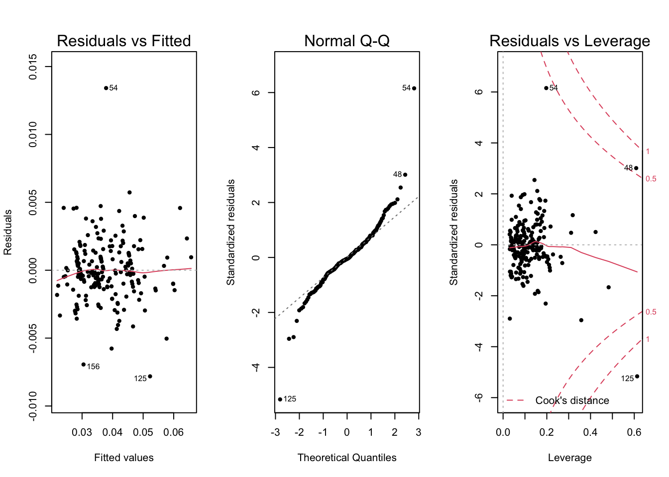
Figure 2.4: Diagnostic plots for Gallons per Mile model
Our new model’s \(R^2\) increases to 0.94 with adjusted \(R^2\) to 0.93, whilst having far less significant heteroscedasticity, residuals more evenly spread around zero, and a better Q-Q plot. This gives us the best of both worlds with a better fitting model which also obeys the modelling assumptions more. A drawback to using this transformation is that our model is no longer predicting the original MPG, but instead the inverse of this: GPM. However, we believe that GPM is still an intuitive idea that can be understood and we can still explain the trend in MPG since an increase in GPM indicates a decrease in fuel efficiency, i.e. MPG.
2.2.2 Outliers and Influential Observations
We do however note some concerning potential outliers. Looking at the Residuals vs Fitted plot on Figure 9, we see that observation \(54\) has an usually large residual, as well as \(125\) and \(156\) to a lesser degree. Further, \(54\) and \(125\) appear as outliers on the Q-Q plot. Lastly, \(48\), \(54\) and \(125\) have a large Cook’s distance which suggests that they may be outliers, influential observations that distort our model, or both. We will keep these observations in mind as we investigate the model further.
We will now consider a “Dffit” plot which shows by how much the predicted value of an observation changes when we fit a new model with that observation removed. Observations which have a large value are observations that are likely influential and distort the model as the large value shows that the model prediction changes significantly when they are not accounted for.
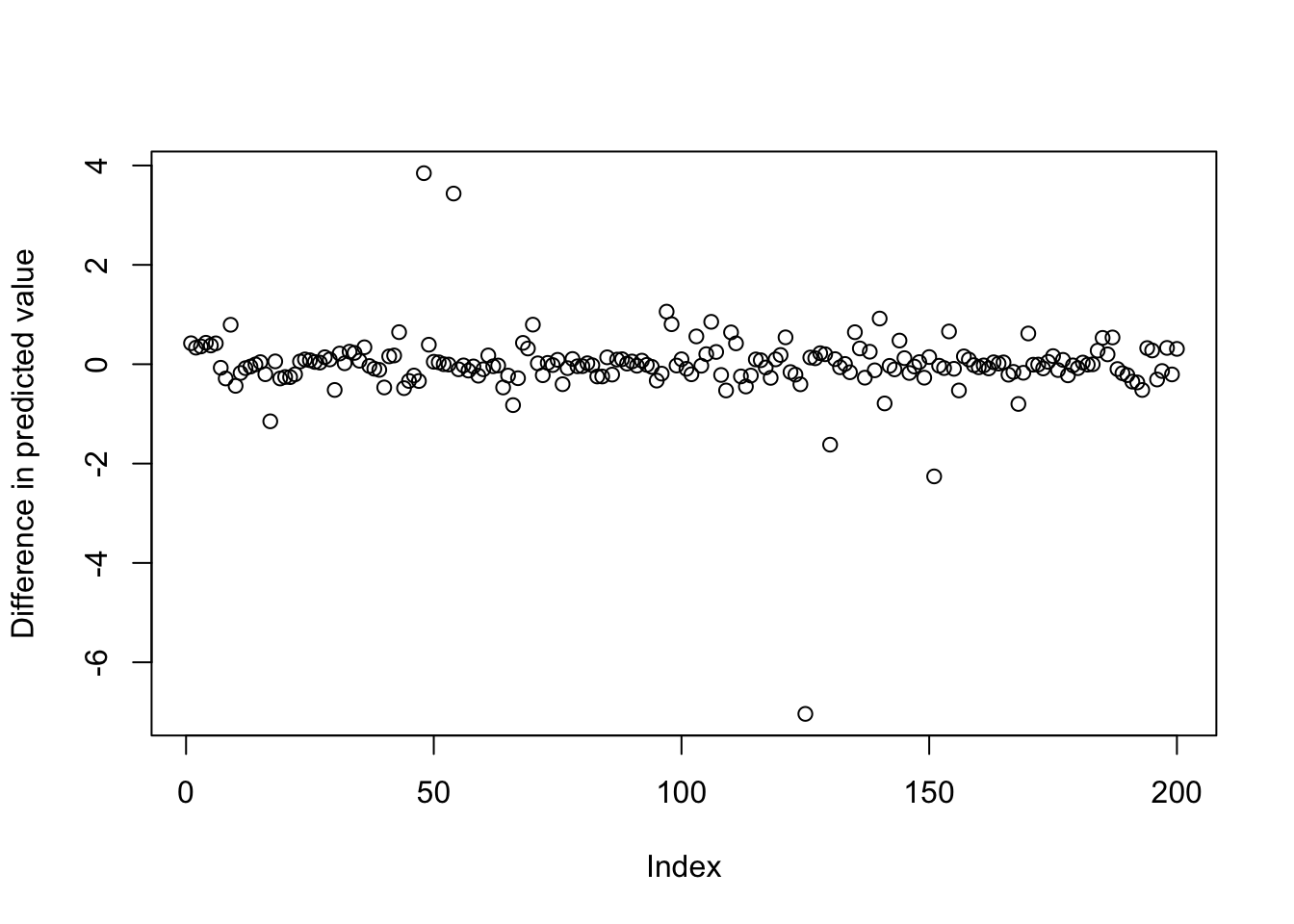
Figure 2.5: Dffits plot showing observations 54 and 125 with large values
In this plot we notice that observations \(54\) and \(125\) appear again. This adds to our concerns that these observations may be affecting the model.
We will also consider “added variable” plots which show how much we can predict the \(GPM\) with a specific variable after accounting for all other variables. These allow us to identify unusual observations and whether an explanatory variable provides useful information in our model. One such variable we will look into is Price. Whilst there is a strong correlation between MPG and Price, it is also reasonable to suspect that Price itself is a function of all the other data available about a car, and so, once other variables have been included, Price itself no longer provides any useful data, so the added variable plot should show no overall trend. Further, if Price were to have an effect, our model would give the conclusion that two otherwise identical cars could have widely different fuel efficiencies if one is sold at a different price to another which is clearly nonsense. However, inspecting the added variable plot for Price we do see a clear trend.
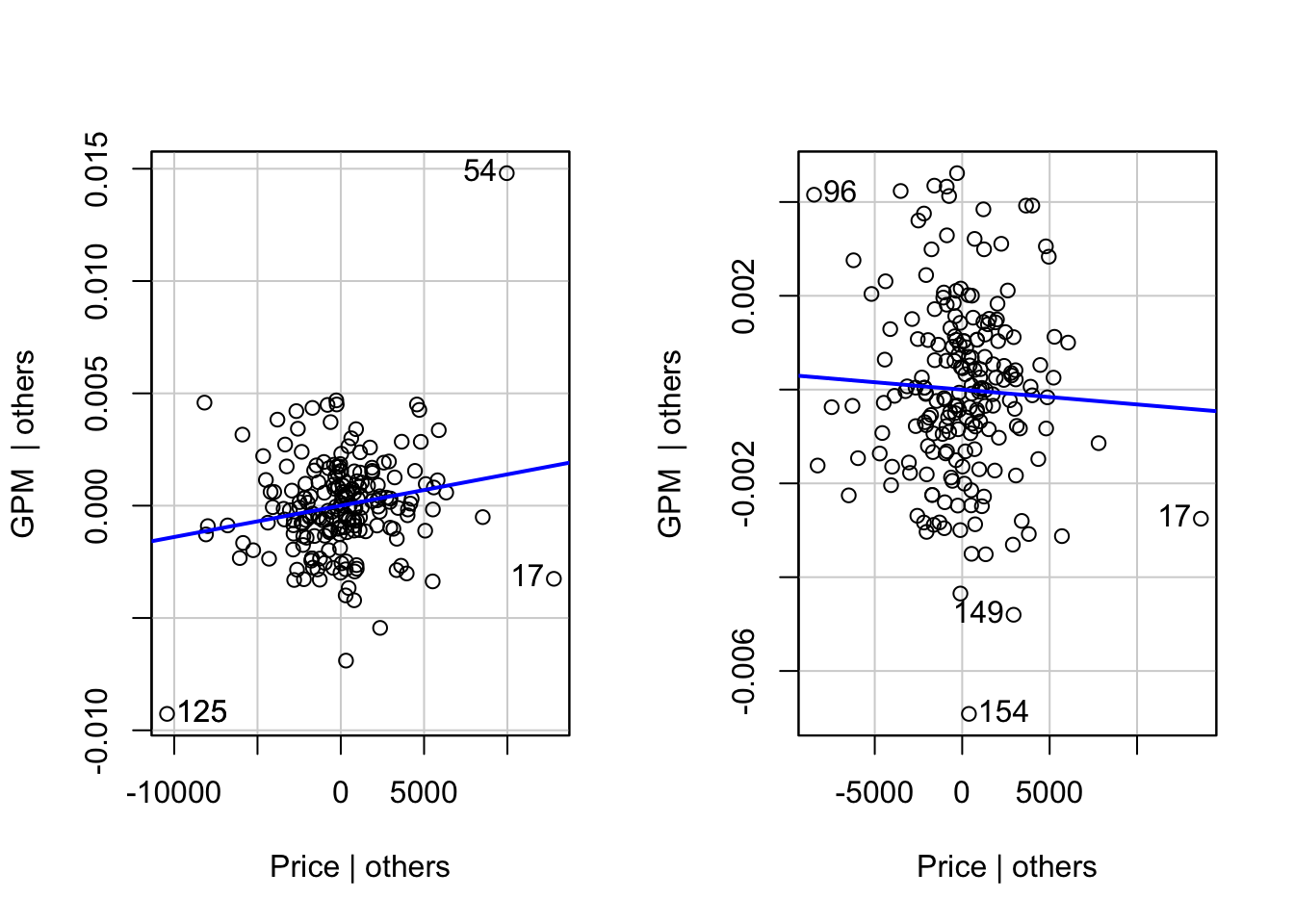
Figure 2.6: Added variables plots
We also notice that observations \(54\) and \(125\) again stand out in this diagram. In particular each point serves to draw the line of best fit towards them and without these points, it appears as if there would be a reduced trend between the \(x\) and \(y\) values. If we remove these observations and refit the model we see that there is a reduced effect of Price on GPM. These two observations were already highly unusual due to their large residual values, position on the Q-Q plot and their large Dffit values. Also, since their inclusion leads us to the strange conclusion that merely changing the price of a car arbitrarily could change its fuel efficiency, we may wish to remove these from the analysis.
Ideally, we would carry out two analyses in parallel, one including these two data points and one excluding, so that we may compare the results. However, in the interests of brevity, we shall only focus on the latter of these two as we find the model that does not suggest that Price has an effect of fuel efficiency more appealing.
2.2.3 Variable Selection
Now that we have decided to remove the most prominent outliers, we wish to see whether a simpler model adequately explains the data. There are certain explanatory variables which, based on prior knowledge about cars, we would expect to not affect the fuel efficiency of the car, and so we will check if a model excluding these variables is no worse than the full model. We have the following variables, with reasons, which we expect to not be important in our model:
- Price - Keeping all other variables constant, the price a car is sold at should not change the fuel efficiency.
- Height, Width, Length, Wheel Base, Body - Dimensions of the car, as its shape (Body), should effect fuel efficiency only though the increased weight for larger cars, which is already accounted for, and drag, which we expect to be small.
- Doors - Keeping all of other variables constant, adding or removing doors should not change fuel efficiency by any appreciable amount.
- Engine Size, Bore - The size of the cylinders (Bore) serve as a factor in determining Engine Size. For engine size, we only expect the size of the engine to effect fuel efficiency through increased weight, which is already accounted for as a variable, and the fact that larger engines tend to be more powerful, which is accounted for by horsepower.
| Res.Df | RSS | Df | Sum of Sq | F | Pr(>F) |
|---|---|---|---|---|---|
| 185 | 0.0007838 | NA | NA | NA | NA |
| 174 | 0.0007174 | 11 | 6.64e-05 | 1.463305 | 0.1492022 |
In the above table, we are primarily interested in the bottom right-most entry which provides the p-value for the hypothesis test. We see that the p-value of \(0.149\) is larger than \(0.05\), hence there is insufficient evidence to suggest that any one of these variables should be included in the model. As such, we remove these variables from our model simplifying it in the process.
For variables which we cannot discount on the same grounds as above (i.e. those that we intuitively think should have no effect), we instead carry out individual nested ANOVA tests to see if certain categories of variables are collectively significant or not, these categories being Drive, Fuel System and Cylidners. We omit the ANOVA results for brevity, but in all cases, the remaining categorical variables were all had a p-value less than \(0.05\) and thus are collectively significant, i.e. we will retain them in the model.
2.3 Final Model
| (Intercept) | DriveFront | DriveRear | CurbWt | FuelSysidi | Stroke | CompRatio | Horsepower | PeakRPM | Cylindersfive | Cylinderssix | Cylinders>=eight | FuelSysidi:CompRatio | |
|---|---|---|---|---|---|---|---|---|---|---|---|---|---|
| Estimate | 25.866 | -0.577 | -0.714 | 0.01 | -48.386 | -1.924 | -2.226 | 0.07 | 0.001 | 3.816 | 0.988 | 8.028 | 3.216 |
| Pr(>|t|) | 0.000 | 0.470 | 0.394 | 0.00 | 0.001 | 0.001 | 0.000 | 0.00 | 0.006 | 0.000 | 0.134 | 0.000 | 0.000 |
Our final model uses the above variables seen in the table (rounded to 3d.p.). Looking at the p-values in the bottom row, we see all are significant at the \(5\%\) level (i.e. there is evidence that we need them in the model) except for the drive variables and cylinderssix. However, as stated earlier, these are collectively significant in their categories following the ANOVA analysis so we keep these in the model as well.
Lastly, to aid in understanding, we multiply through by a factor of \(1000\) to obtain a model for gallons per \(1000\) Miles. This increases the size of the parameter estimates making them easier to interpret, but otherwise does not affect the inferences of our model (for example, the p-values all remain the same).| R2 | Adjusted R2 | |
|---|---|---|
| Final Model | 0.951 | 0.951 |
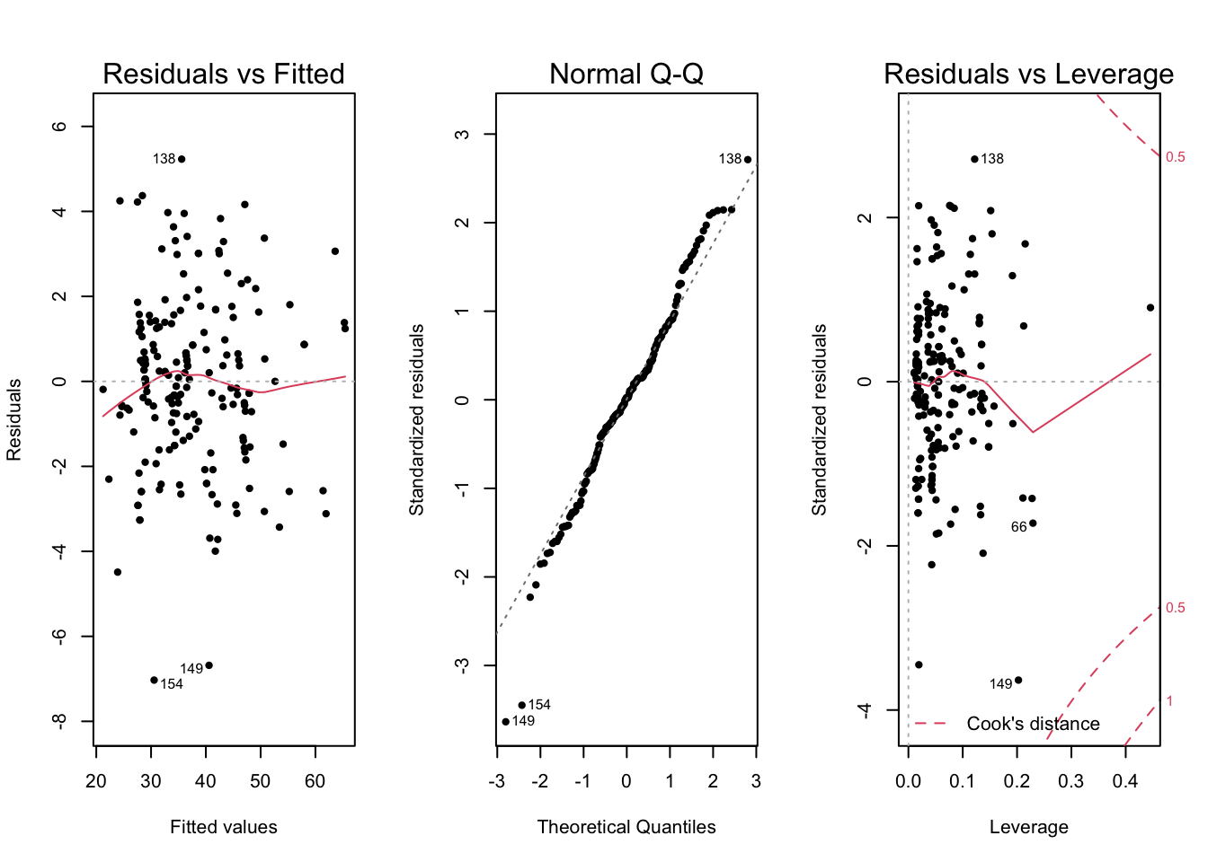
Figure 2.7: Diagnostic plots for the final model
The diagnostic plots of our final model help to confirm the validity of our model. The Residuals vs Fitted plot exhibits little to no heteroscedasticity and our Q-Q plot very closely follows the straight line for all but two observations. Also, the Cook’s distance plot shows there are no observations that cause significant concern as no observation is close to the \(0.5\) contour which indicates outliers/potentially influential observations. As a result, we are confident that the model assumptions are being fulfilled and there are no influential observations that are distorting the model. In a further analysis we may wish to investigate the two observations that demonstrate relatively large residuals, but as they do not appear to be influential on the Cook’s distance plot, we do not believe they are distorting the model and negatively affecting our inferences or model predictions.
2.4 Model Explanantion
After our analysis, we have now obtained a statistical model that can be used to predict the fuel efficiency of the car. Our model predicts the fuel efficiency of a car through the number of gallons needed to drive one thousand miles, which we denote as \(GPTM\).
\[\begin{align*} \hat y_{GPTM} &= 25.9 -0.577x_{\textrm{FrontWhlDrv}} -0.714x_{\textrm{RearWhlDrv}} +0.00984x_{\textrm{CurbWgt}} \\ &-48.4x_{\textrm{idiFuelSys}} -1.92x_{\textrm{Stroke}} -2.23x_{\textrm{CompRatio}} +0.0696x_{\textrm{Horsepower}} \\ &+0.00118x_{\textrm{PeakRPM}} +3.82x_{\textrm{5Cyl}} +0.988x_{\textrm{6Cyl}} +8.03x_{\textrm{>8Cyl}} +3.22x_{\textrm{idiCompRatio}} \end{align*}\]
To make a prediction, we consider the values of these variables for a car and plug them into the above formula. For properties of a car that are numbers, for example the horsepower, we plug in the horsepower value directly. For properties of a car that are either true or false, we set the relevant \(x\) term in the above equation to \(1\) and the rest to \(0\). So for example, if a car has front wheel drive, we set \(x_{\textrm{FrontWhlDrv}}\) to \(1\) and \(x_{\textrm{RearWhlDrv}}\) to \(0\). If a car has 4-wheel drive, we set both to \(0\). Lastly, the \(x_{\textrm{idiCompRatio}}\) term is unique in a sense that it takes the same value of the compression ratio of the car if it has an idi fuel system, and \(0\) otherwise.
After putting in all the relevant values we can obtain a prediction for the fuel efficiency of the car in terms of the gallons per 1000 Miles. To get a value for Miles per Gallon instead, we can divide the output of our model by \(1000\) and take the reciprocal. So for example, if we obtain a prediction of \(50\) from our model, we divide \(50\) by \(1000\) to obtain \(0.05\), then take the reciprocal \(\frac{1}{0.05}=20\) to obtain our prediction for the Miles per Gallon of the car.
Our earlier analysis shows that this is highly accurate, with our model able to explain over \(95\%\) of the variation of the original data. Intuitively, this means that, in a certain sense, we are less than \(5\%\) off from a perfect prediction of the \(GPTM\) value of a car.
If we wish to produce a car with greater fuel efficiency, i.e. a greater MPG value, we wish to decrease the gallons used per single mile, or equivalently the GPTM value. To decrease the GPTM value we need to reduce the value of any property of the car that is being multiplied by a positive value, and decrease the value of any property that is being multiplied by a negative value. For example, if we increase the stroke of the car, the GPTM will go down, and if we increase the Horsepower, the GPTM will go up. It is important to keep in mind however that increasing one value may require us to decrease another to accommodate.