Bankruptcy
 Photo by Towfiqu Barbhuiya on Unsplash
1 Introduction and Data Preprocessing
This report aims to investigate the subset of a financial dataset, , introduced from the UCI Repository by Tomczak et al. (2016). With the help of a logistic regression model, we try to predict the probability of company bankruptcy in terms of various financial indicators.
PolishBR contains 291 missing values. After closer inspection, we discovered that cost of products sold (CostPrS) and current liabilities (CLiabil) are missing together in 266 observations. The remaining missing values also seem to be missing together with other variables. That indicates that these are not missing at random, and we cannot use any imputation method on them.
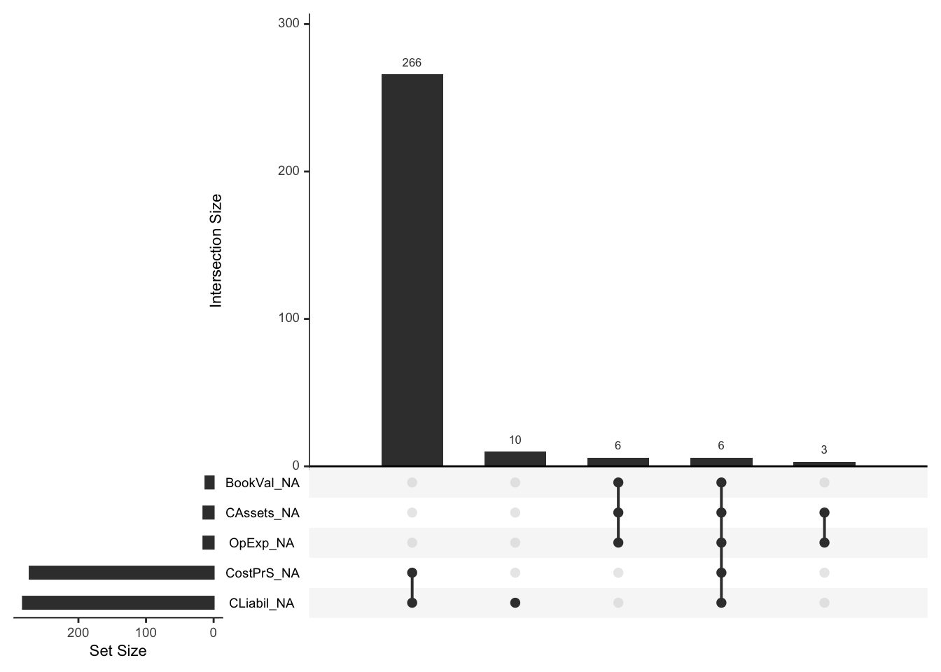
Figure 1.1: Missing values
However, noting the size of our data, we can safely ignore these values altogether. However, further investigation would be essential because the proportion of companies that went bankrupt in the data made of observations containing some missing information is about 0.127, while in the complete data it is only about 0.061.
After removing missing values, we end up with 5218 observations of 11 variables, two of which are categorical (factor type).
2 Explanatory Data Analysis
2.1 Preliminaries
The distributions of numerical predictors are highly skewed to the right and contain multiple extreme outliers. Naturally, we expect some unusually high values in the tail of distributions. However, there is one suspicious observation that looks more like a mistake considering other values of this variable:
| bust | TAssets | TLiabil | WkCap | TSales | StLiabil | CAssets | OpExp | BookVal | CostPrS | CLiabil |
|---|---|---|---|---|---|---|---|---|---|---|
| 0 | 5.961368 | -2568.575 | Low | 391.1075 | 69.77781 | 31.27302 | 382.3126 | 2025.989 | 382.311 | 78.91632 |
Since we cannot determine the nature of such a high negative value of total liabilities (TLiabil), we decided to discard this observation.
After the literature review, we found out that the book value of equity (BookVal) can be calculated by subtracting total liabilities from total assets, i.e. \[\begin{align*} \text{Book value of equity} = \text{Total assets} - \text{Total libilities}. \end{align*}\] Indeed, these values look alike (accounting for the rounding error and few unusual observations). Table 2.2 displays the difference between BookVal and a variable calculated according to the formula above.
| Min. | 1st Qu. | Median | Mean | 3rd Qu. | Max. |
|---|---|---|---|---|---|
| -1911.97 | -1.67 | 0 | -3.04 | 0 | 0.14 |
Furthermore, the working capital (WkCap) can be calculated by subtracting current liabilities (CLiabil) from current assets (CAssets). However, since we are given categorical labels for this variable, we decided to retain it in its original form.
A word on current liabilities
The data does not provide any explanation of the difference between current and short-term liabilities. Many sources use these terms interchangeably to quantify financial accountabilities to be settled within the fiscal year of the operating cycle. However, plotting these variables against one another shows almost perfect alignment up to some point where the pattern breaks. Furthermore, one would expect the current liabilities to be part of total liabilities - similarly, current assets to be included in total assets. Even though the data supports the latter, it does not justify the former. Nonetheless, short-term liabilities do behave as expected concerning total liabilities, and therefore, we believe they are more reliable in our analysis. From now onwards, unless otherwise stated, we shall treat short-term liabilities (StLiabil) as current liabilities and use these terms interchangeably.
2.2 Variables Ralationships
The percentage of companies that went bankrupt split by their working capital is presented in Table 2.3. 16% of companies with low working capital became insolvent. This number drastically decreases for medium, high and very high working capital, suggesting that this variable could be a valuable predictor.
| Low | Medium | High | Very High | |
|---|---|---|---|---|
| 0 | 84 | 95.1 | 97.1 | 98.94 |
| 1 | 16 | 4.9 | 2.9 | 1.06 |
2.2.1 Correlation
It is always a good practice to examine the correlation between explanatory variables. Figure 2.1 shows the correlation plots for raw and transformed variables. To produce the second plot, we used log-transformation on all numerical predictors, but BookVal, which for now, has been discarded. We can see how the extreme outliers impact the correlation (especially CostPrS and CLiabil) and how a simple transformation can reduce their effect.
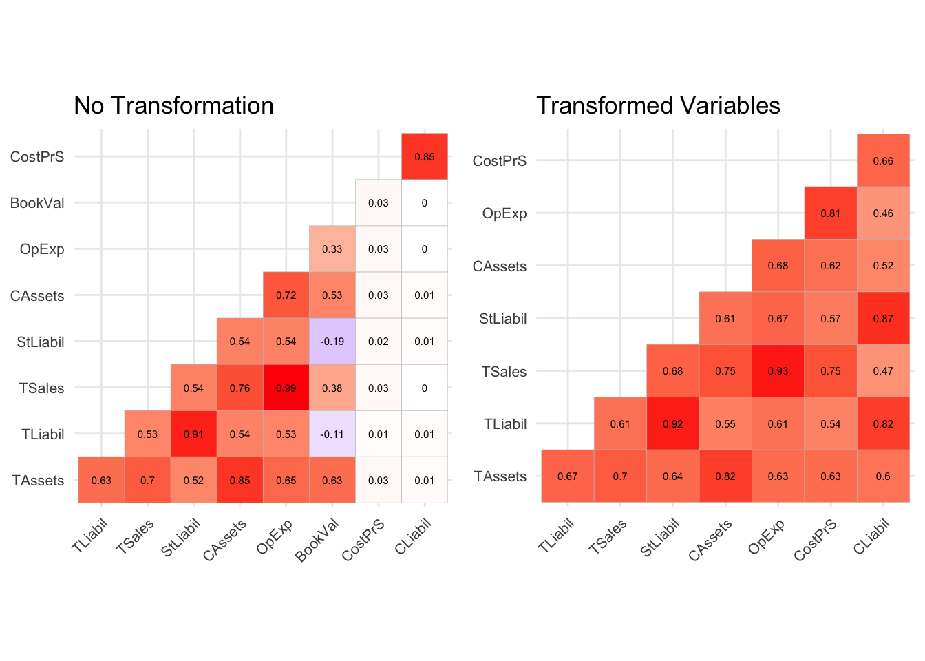
Figure 2.1: Correlation plots
Not surprisingly, the correlation between liabilities and assets (be it current, short-term or total) is high. We note an almost perfect correlation between operating expenses (OpExp) and total sales (TSales). Plotting these variables does not reveal much. However, we may reason that as the company grows, it produces and sells more goods (high TSales), and its operating expenses tend to increase accordingly. Therefore, in this case, the company’s size might be a lurking variable responsible for such a strong correlation between these variables. Perhaps unexpectedly, operating expenses and the cost of products sold are highly correlated. It turns out that in about 60% of observations, operating expenses observations are almost identical (+-1) to the cost of products sold (correlation of 0.999). Data does not give any indication of why such a perfect relationship exists.
2.2.2 Short and Long-Term Obligations
Let introduce a measure helping us quantifying companies liquidity (ability to pay debts as when they fall due): \[\begin{align*} \text{Current ratio} = \frac{\text{Current Assets}}{\text{Current liabilities}}. \end{align*}\] A ratio lover than 1 suggests that short-term (within one fiscal year) liabilities are greater than accessible assets. Next, we investigate the relationship between going bankrupt and the current ratio. Table 2.4 displays the percentage of companies that went bankrupt and had the current ratio below or above 1. We can see that almost 17% of companies, having a ratio lower than 1, became insolvent.
| Ratio_Below_1 | Bust | Percent_bust |
|---|---|---|
| no | no | 96.46 |
| no | yes | 3.54 |
| yes | no | 83.07 |
| yes | yes | 16.93 |
To measure companies capabilities to meet their long-term financial obligations, consider the following metric: \[\begin{align*} \text{Shareholder Equity Ratio} =\frac{\text{Book value of equity}}{\text{Total assets}}. \end{align*}\] Hight Equity Ratio indicates that the company effectively manages its finances, and therefore, it will be able to meet its long-term financial liabilities Companies with Shareholder Equity Ratios bigger than 0.5 are considered conservative because they rely mainly on the stakeholders’ equity rather than on debt. On the other hand, a company with a ratio smaller than 0.5 has a substantial amount of debt in its capital structure - it is called a leveraged company. If the ratio is considerably small, the company’s financial liabilities might outweigh its income.
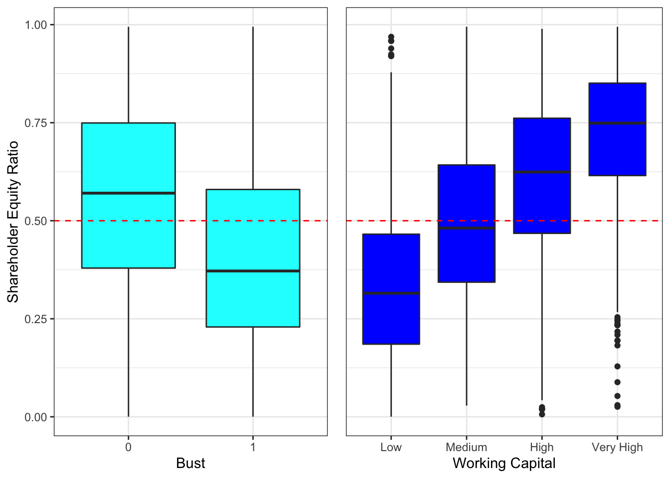
Figure 2.2: Equity ratio relationships
We can see that companies that went bankrupt tend to have smaller Shareholder Equity Ratios and low-to-medium working capital. This observation indicates that the ratio could help determine the likelihood of becoming bankrupt. The negative Equity Ratio is an indication of financially dangerous struggles. It is, therefore, no surprise that among 246 companies with a negative ratio, over 28% became insolvent.
2.2.3 Remaining Predictors
So far, we have investigated how assets, liabilities and their combination, such as equity ratio, can be used to explain a company’s finances and impact the probability of a company going bankrupt. We are left with three predictors to examine. Consider Figure 2.3 showing log-transformed variables plotted against log odds ratio. We can see that for all cases, the variable’s values increase results in a (more or less apparent) decrease in log odds ratio, that is, the lower the odds of a company going bankrupt. This decrease is the most evident for total sales. Intuitively, more sales imply more income and more financial stability. It is less obvious why operating expenses and the cost of goods sold can decrease the odds ratio. As mentioned earlier, we suspect that these measures indicate the company’s size and growth, generally speaking. Therefore, it may explain the present trends. Plotting log odds ratio against current or total liabilities, however, presents the opposite relation - the bigger the debt and financial obligations, the bigger the chance of going bankrupt.
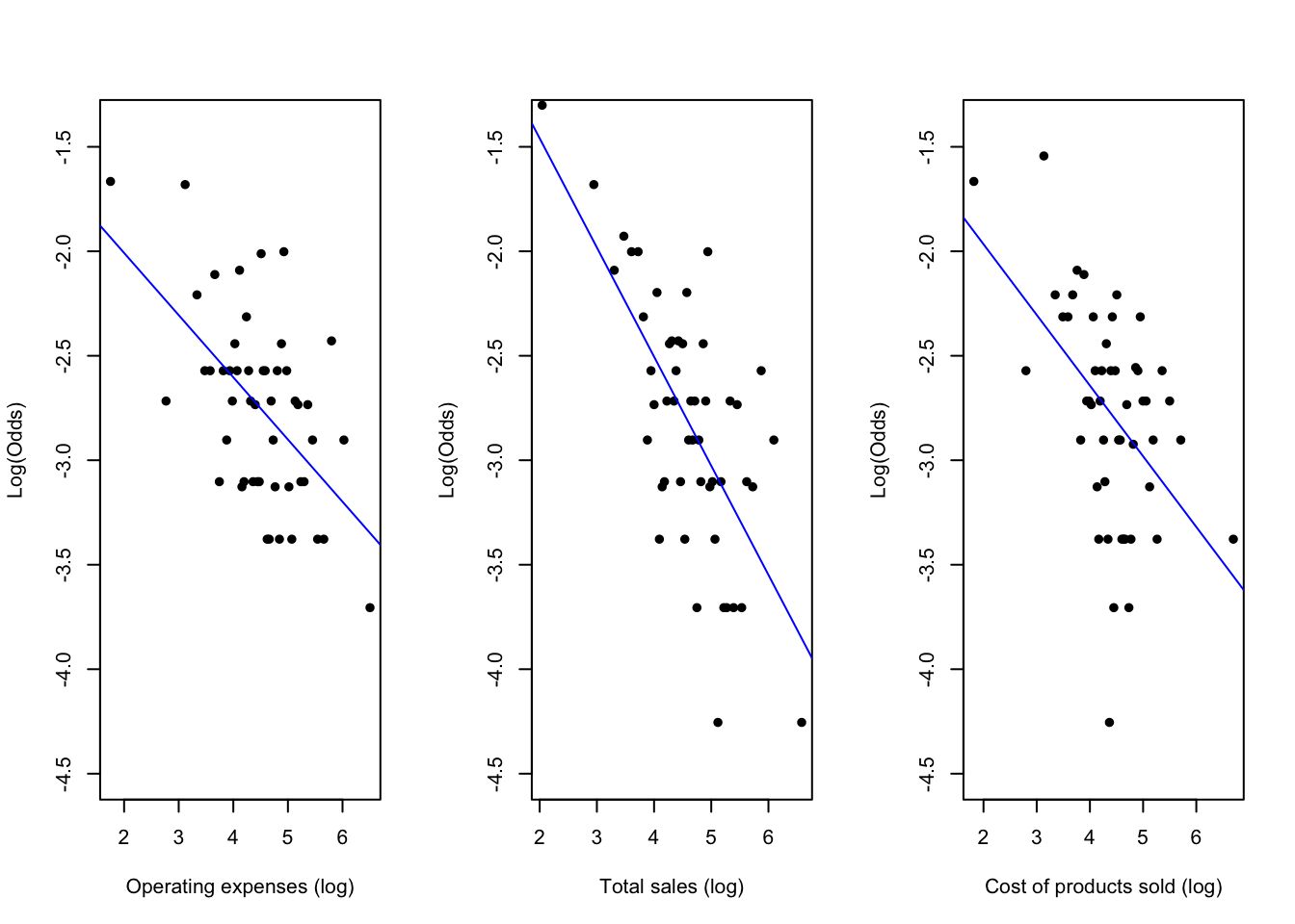
Figure 2.3: Remaining predictors
3 Modelling
3.1 Class Imbalance
Before we begin the modelling, it is crucial to address a critical issue our data exhibits, namely the class imbalance. As noted in the EDA, companies that went bankrupt constitute only about 6.1% of the dataset. That means this category is rare, and the logistic regression model will struggle to predict this particular outcome. If we do not find a solution taking into account this fact, predicting non-bankruptcy will always be better, in terms of accuracy, than predicting insolvency. The context is of vital importance here. Failing to predict bankruptcy is far more dangerous than anticipating it where it will not actually occur. The model’s predictions could be used as a precaution, and the company could take appropriate measures regardless of the outcome. We can translate this scenario into the model’s sensitivity and specificity. Here, we are willing to sacrifice some specificity (predicting a company going bankrupt when it fact it will not) in order to increase sensitivity (forecasting a company not going bankrupt when, in fact, it will). As logistic regression returns predicting probabilities vector, a question now arises: how do we decide on the optimal probability threshold for assigning an observation to either class?
3.1.1 The Need of Validation Set
We use the following steps to find the best logistic model. First, we created dummy variables from the WkCap variable with the baseline Low level. Then, the data was split into three subsets - training, validating and testing set (in proportions 0.7, 0.15 and 0.15, respectively). We ensure that each set contains the same proportion of companies that went bankrupt (Bust = 1) by utilising the caret package and createDataPartition function. All proposed models learn on the training set. Then, using the validation set, we find the optimal probability cutoff for the binary classification. To do that, we plot the model’s sensitivity and specificity against the probability thresholds and find a value for which they coincide. A similar procedure is implemented for all proposed models. Finally, we compare models’ class predictions on the testing set to choose the best performing model.
3.2 Model Selection
3.2.1 Proposed Models
We have trained the following models:
Model_Base: The first model includes all predictive variables without any transformation or altering - this will serve as the base simple model for comparison.Model_Red_Back: To fit this model, we take advantage of the findings from explanatory data analysis. First, we account for the right skeweness of numeric predictors by using the log transformation. By the discussion in Section 2.1, we replace BookVal by its proper definition, and discard CLiabil. We also add two ratios defined in Section 2.2.2. Finally, we reduce the initial model using automated stepwise selection method (at 5% significance level).Model_Red_LASSO: Reduce the initial model (the same as forModel_Red_Back) using LASSO method.
3.2.2 Backward Selection
Let us breifly explain how the backward selection method works. In each step we inspected tests’ p-values and locate the highest one. These numbers provided us with indication whether a variable is needed in a model or not. For example, consider an initial full model trained on all the explanatory variables:
| LR Chisq | Df | Pr(>Chisq) | |
|---|---|---|---|
| BookVal | 2.8124580 | 1 | 0.0935350 |
| WkCap_Medium | 17.7609456 | 1 | 0.0000250 |
| WkCap_High | 10.8656209 | 1 | 0.0009797 |
| WkCap_Very_High | 12.2031590 | 1 | 0.0004771 |
| CRatio | 3.1352778 | 1 | 0.0766153 |
| ERatio | 0.4024692 | 1 | 0.5258168 |
| log_TAssets | 1.5626008 | 1 | 0.2112848 |
| log_TLiabil | 0.3936412 | 1 | 0.5303916 |
| log_TSales | 60.2769767 | 1 | 0.0000000 |
| log_StLiabil | 3.3798478 | 1 | 0.0659981 |
| log_CAssets | 2.3323638 | 1 | 0.1267093 |
| log_OpExp | 54.4311741 | 1 | 0.0000000 |
| log_CostPrS | 0.3844665 | 1 | 0.5352225 |
We can see that the p-value for log_CostPrS is the biggest of them all. That means we have evidence to think it is equal to zero, and therefore, to remove it from the model. Next, we fit the model again, but without log_CostPrS, and discard another variable with the biggest p-value. The process continues until we obtain only substantial predictors, that is, variables for which we have strong evidence (in terms of p-value) that are needed in the model. In our case, such predictors are summarised in table below.
| (Intercept) | BookVal | WkCap_Medium | WkCap_High | WkCap_Very_High | log_TAssets | log_TSales | log_OpExp |
|---|---|---|---|---|---|---|---|
| -0.8033 | -0.0083 | -1.1994 | -1.2588 | -1.7954 | -0.3177 | -3.6474 | 3.7647 |
Coefficients interpretation
We can interpret any coefficient from Table 3.2. For example, consider BookVal coefficient. Its number means that an increase of book value of equity by one unit, while keeping other variables constant, results in the odd ratio of \(\exp(-0.0083)=0.9917\), i.e. the odds of going bankrupt decrease by less than 1%. Similarly, for the WkCap_Very High coefficient, \(\exp(-1.7954)=0.1661\), i.e. the odds of going bankrupt for campnies with high working capital decrease by 83.4%. According to this model, only operating expenses increase the odds of going bankrupt - this suggests reevaluation, or reconsidering the model bearing in mind findings from the EDA.
3.2.3 LASSO Method
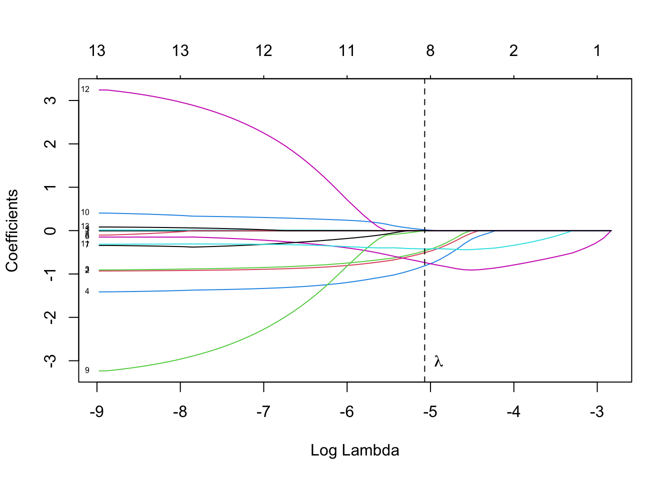
Another way to reduce the full model is the shrinkage approach. Using the LASSO method we aim to minimise \[\begin{align*} \sum_{i=1}^{n} (y_i-\bf{x}^{T}_i\hat{\bf{\beta}})^2+\lambda\sum_{j}^{p} |\hat{\beta_j}| \end{align*}\] i.e. we impose extra condition on the parameter estimates to shrink the model. Commonly, we use cross-validation to choose the optimal \(\lambda\) which can be realised by function in package . However, we obtain different results for the final model if we repeat this process several times, which means instability of the final result by this method. To address this issue, we use bootstrap, repeating the procedure 100 times to find the average of optimal lambdas, which should stabilise the model. Then we plot the trace to ensure the reasonability of this choice.
3.2.4 Optimal Probability Cutoffs
We exploit the validation set to find the optimal probability thresholds for each of the models. By using the same validation set for all models we ensure a fair decision on the best performing model, i.e. choosing an optimal cutoff values will not interfere with predictions on the testing set.
Let us assess each model on the validation set. Figure 3.1 presents the sensitivity and specificity values of Model_Red_Back for different probability thresholds.
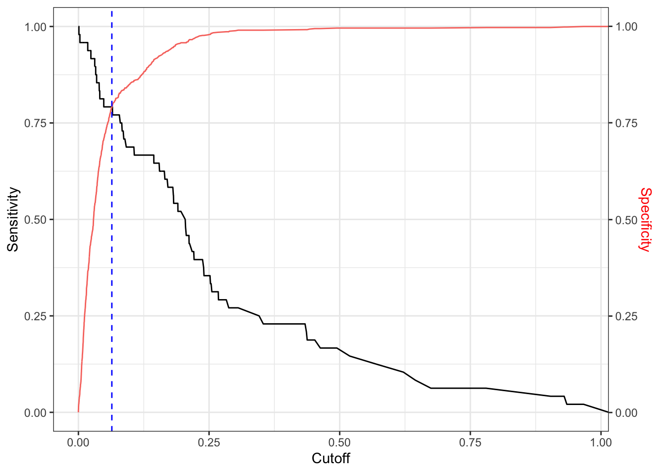
Figure 3.1: Optimal probability cutoff
The blue dashed line indicates the optimum. Note that if we used default classification probability of 0.5, model’s accuracy would increase to almost 0.95 with extremely high specificity - 0.99, but disappointingly poor sensitivity - only 0.15. Accuracy, in such a case, would be artificially inflated and the model would be unreliable. This is because accuracy-wise, it is better to always predict that a company will not go bankrupt. In a similar way, we find the optimal probability threshold for Model_Red_LASSO.
3.2.5 Models Comparison
Table 3.3 summarises some of the performance metrics for all four models.
| Model_Base | Model_Red_Back | Model_Red_LASSO | |
|---|---|---|---|
| Accuracy | 0.948 | 0.754 | 0.706 |
| Kappa | 0.241 | 0.199 | 0.168 |
| Sensitivity | 0.149 | 0.787 | 0.830 |
| Specificity | 0.999 | 0.752 | 0.698 |
| Parameters | 13.000 | 8.000 | 9.000 |
We can see that even though Model_Base seems highly accurate, its low sensitivity makes it worthless. Kappa is a better metric in assessing model fit in a case of class imbalance. It suggests our models fit the data only slightly. Nevertheless, Model_Red_Back looks the best accounting for all metrics.
4 Further Analysis
Some additional work could include:
- Proper investigation for data with missing values.
- Other methods for dealing with class imbalance, such as SMOTE algorithm, could be implemented and compared with our models.
- More carefull examination of extreme values.
- More extensive data analysis - perhaps consulting with a specialist would shed light on some patterns we may have missed in our analysis.
- Adding interactions and/or non-linear terms.
- Trying different models, e.g. random forest or kNN.