Loss and Risk

Suppose we know the predictors $X\in \mathcal{X}$, and we wish to make accurate predictions of $Y\in \mathcal{Y}$, i.e. $X$ and $Y$ are random variables (or vectors) that have outcomes in $\mathcal{X}$ and $\mathcal{Y}$ respectively. We can translate the intuition behind “how well a model does” by investigating how off it is from predicting the actual observations. Let’s say we have some function $f\in \mathcal{F}$ that takes predictors as its input and outputs the predictions, i.e. $f:\mathcal{X}\mapsto \mathcal{Y}$. Then a loss function “rewards” our function if it predicts the outcome close to the actual, or “punishes” it when it is far from the truth. This reward-punish strategy translates into assigning an appropriate (positive) value - a score, i.e.  $$\begin{array}{r}L:\mathcal{Y}\times \mathcal{Y}\mapsto {\mathbb{R}}^{+}\end{array}$$ To put it simply, a loss function measures the overall difference between predictions and reality - we want this difference to be as little as possible. What if we gave $f$ different predictors $X$? How about different outcomes $Y$? We wish to know how our model performs on average over different $X$ and $Y$ - this is where the risk comes in, let’s creatively call it $R$. In other words, $R:\mathcal{F}\mapsto {\mathbb{R}}^{+}$ is given by $$\begin{array}{r}R(f)={\mathbb{E}}_{X,Y}[L(Y,f(X))].\end{array}$$

Squared error loss and the optimal risk

One of the most common loss functions is the squared error loss. As the name suggests, it is simply the square of the difference between $Y$ and predictions $f(X)$, i.e. $$\begin{array}{r}L(Y,f(X))=(Y-f(X){)}^2\end{array}$$ How does the risk look like under this function? $$\begin{array}{r}R(f)={\mathbb{E}}_{X,Y}[L(Y,f(X)]={\mathbb{E}}_{X,Y}[(Y-f(X){)}^2]={\mathbb{E}}_X[\underset{\text{consider first}}{\underbrace{{\mathbb{E}}_Y[(Y-f(X){)}^2|X]}}]\end{array}$$ (where we used the fact that $\mathbb{E}[Y]=\mathbb{E}[\mathbb{E}[Y|X]]$, the towering property of expectations). We have $$\begin{array}{rl}{\mathbb{E}}_Y[(Y-f(X){)}^2|X]& ={\mathbb{E}}_Y[Y^2-\underset{\text{not depend on }Y}{\underbrace{2f(X)}}Y+\underset{\text{not depend on }Y}{\underbrace{f(X{)}^2}}|X]\\ & ={\mathbb{E}}_Y[Y^2|X]-2f(X){\mathbb{E}}_Y[Y|X]+f(X{)}^2\\ & ={\mathbb{E}}_Y[Y^2|X]\underset{\text{subtract and add the same thing}}{\underbrace{-({\mathbb{E}}_Y[Y|X]{)}^2+({\mathbb{E}}_Y[Y|X]{)}^2}}-2f(X){\mathbb{E}}_Y[Y|X]+f(X{)}^2\\ & ={\mathrm{Var}}_Y[Y|X]+({\mathbb{E}}_Y[Y|X]-f(X){)}^2.\end{array}$$ That can already tell us a lot! Notice that whatever function $f$ we consider, we will always end up with a variance term that is completely independent of it, i.e. there is the irreducible error due to the randomness in $Y$ that cannot be captured by $f$. We can never predict perfectly unless there is a deterministic relationship between $X$ and $Y$. Coming back to the risk $$\begin{array}{r}R(f)={\mathbb{E}}_X[{\mathrm{Var}}_Y[Y|X]]+{\mathbb{E}}_X[({\mathbb{E}}_Y[Y|X]-f(X){)}^2].\end{array}$$ we can ask what the best $f$ we can come up with is? Well, it is equivalent to asking which $f$ minimises the risk. It is easy to see that the second term becomes zero when $$\begin{array}{r}{f}^{\ast }(X)={\mathbb{E}}_Y[Y|X].\end{array}$$ This is the optimal solution.

Empirical Risk

All is nice and clear, and we have our solution. However, we do not know the joint distribution of $X$ and $Y$, and therefore, finding the risk and exact function is impossible. So what is the solution? Our data! Let’s call it $\mathcal{T}=\{(X_i,Y_i){\}}_{i=1}^n$ - $n$ realisations of random variables (or vectors) $X$ and $Y$. The natural metric we can use instead of the acutal average is the empirical average - and this is how we define the empirical risk $$\begin{array}{r}\hat{R}(f)=\frac{1}{n}\sum _{i=1}^{n}L(Y_i,f(X_i)).\end{array}$$ The law of large numbers ensures that when the sample size increases, $\hat{R}(f)$ approaches the “true” risk $R(f)$ for any $f\in \mathcal{F}$.

Set up

Suppose the “true” function (in reality not available to us) of one predictor is
$$\begin{array}{r}{f}^{\ast }(x)={(x-2)}^2(x-1)x(x+1).\end{array}$$ Now, we create an artificial sample of 450 observations from $f^{\ast }$ (for $x$ between -1 and 2). We add random noise from the normal distribution of mean zero and variance 1 to each observation. Then we plot the sample and the “true” function used to generate it.

library(tidyverse)
f_star = function(x){return((x-2)^2*(x-1)*x*(x+1))}
set.seed(1)
x = runif(450, -1, 2)

observations = f_star(x) + rnorm(450, 0, 1)

sample = data_frame('x' = x, 'y' = observations)
true_values = data.frame('x' = x, 'y' = f_star(x))
  
ggplot(sample, aes(x, y, colour = "Sample")) + 
  geom_point(alpha = 0.5, shape = 20) + 
  geom_line(data = true_values, aes(colour = "f*(x)")) + 
  scale_colour_manual("", 
                      breaks = c("Sample", "f*(x)"),
                      values = c("black", "blue")) + 
  theme_bw() +
  labs(title = "The sample and the true function") +
  theme(plot.title = element_text(hjust=0.5), legend.position = "top")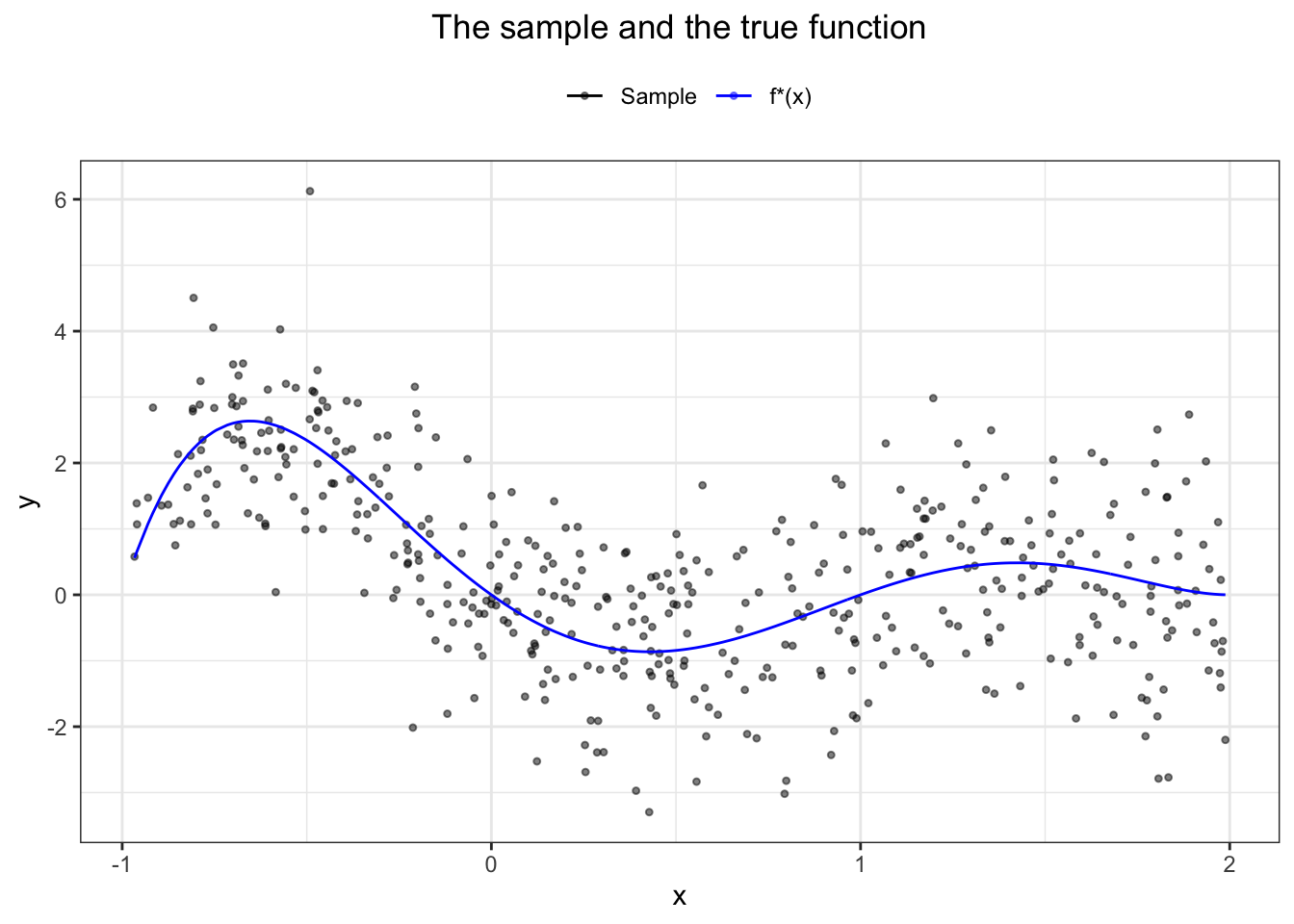

What is the estimated risk of $f^{\ast }$ under the squared loss function? We use the formula above: $$\begin{array}{r}\hat{R}(f^{\ast })=\frac{1}{n}\sum _{i=1}^n(Y_i-f^{\ast }(X_i){)}^2\end{array}$$

sum((sample$y - f_star(sample$x))^2) / length(sample$x)

## [1] 1.099824

This number is not coincidental. Previously, we showed the existence of the irreducible error due to randomness in $Y$ - in our case, this randomness has been added artificially as a random noise with variance 1 - hence we obtain approximately this value.

How do the prediction error change when the complexity of the model changes?

Model Complexity

Imagine that we do not know $f^{\ast }$ and wish to discover it using polynomial regression - a more realistic scenario. We observed the data , and we will use a part of it (training set) to develop a model and the remaining data to see how it performs (testing set). Let’s use the first 40 observations to train the model.

We train 11 models of increasing complexity, starting from a model of just an intercept up to the one with terms up to and including $x^{10}$.

train = sample[1:40, ]
test = sample[41:450, ]

# Getting empirical risks given a regression 
get_errors <- function(reg){
  pred_test <- predict(reg, test[,1])

  train_error <- sum((reg$residuals)^2) / 40
  test_error <- sum((test[,2] - pred_test)^2) / 410
  
  return(c(train_error, test_error))
}

# These will store our outcomes
training_outcomes = c()
testing_outcomes = c()

# Regression with just an intercept
reg0 <- lm(y ~ (1), data = train)
training_outcomes[1] = get_errors(reg0)[1]
testing_outcomes[1] = get_errors(reg0)[2]

# Polynomial regressions of increasing complexity
for (i in 1:10){
  reg <- lm(y ~ poly(x, i), data = train)
  training_outcomes[i+1] = get_errors(reg)[1]
  testing_outcomes[i+1] = get_errors(reg)[2]
}

complexity <- seq(0,10)

outcomes = data.frame(cbind(complexity, training_outcomes, testing_outcomes))

# Plot the results
ggplot(outcomes, aes(complexity, training_outcomes, colour = "Training")) + 
  geom_line() +
  geom_line(aes(complexity, testing_outcomes, colour = "Test")) + 
  theme_bw() +
  scale_x_continuous(labels = as.character(complexity), breaks = complexity) +
  labs(title = "Prediction error against model complexity",
       x = "Complexity", y = "Prediction Error")+
  theme(plot.title = element_text(hjust=0.5), legend.position = "top") +
  geom_text(x = 1.5, y = 2, label = "Underfit", inherit.aes = FALSE) +
  geom_text(x = 9, y = 2, label = "Overfit", inherit.aes = FALSE) +
  geom_text(x = 5, y = 1.5, label = "Optimal", inherit.aes = FALSE, colour = "red") +
  geom_vline(xintercept = 5, linetype = "dashed", colour = "red", size = 0.25) +
  scale_colour_manual("", 
                      breaks = c("Training", "Test"),
                      values = c("blue", "yellow"))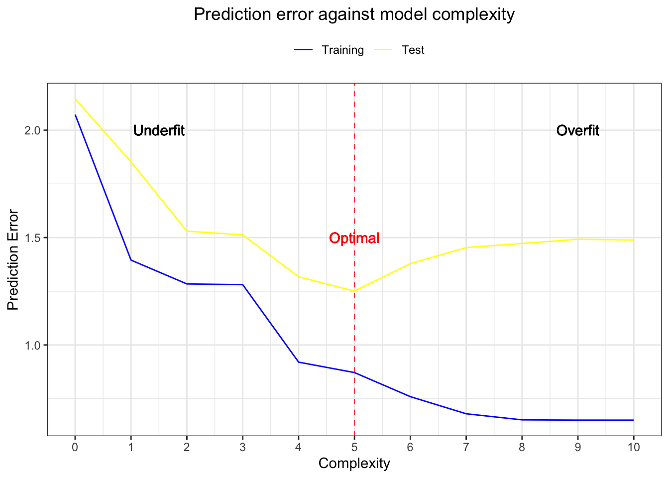 

When the models’ complexity is low, we can see that both the training and testing sets generate significant errors. The model is not complex enough to capture the patterns in our data, i.e. we underfit. The more complex the models become, the smaller the errors on the training set - we fit the data more and more until we fit perfectly (including the noise, which is, of course, undesirable). On the other hand, the errors of the testing set become smaller up to the optimal point, where they start to increase again because our model fits the noise and does not generalise well, i.e. we overfit the data.

The middle area is the sweet spot - the balance between accurate training fit and good generalisation over the testing set. It is therefore not surprising that the best performing model (giving the smallest test error) is the one of order 5 - the same as our “true” function $f^{\ast }$.

Let’s see how our newly found regression compares to the actual $f^{\ast }$.

best_reg_points <- data.frame('x' = sample$x, 
                              'y' = lm(y ~ poly(x, 5), data = sample)$fitted.values)

ggplot(train, aes(x, y, colour = "Training points")) + geom_point(alpha = 0.5) + 
  geom_point(data = test, aes(x, y,  colour = "Test points"), alpha = 0.5) +
  geom_line(data = best_reg_points, aes(x, y, colour = "Best model")) +
  geom_line(data = true_values, aes(x, y, colour = "f*(x)")) + 
  theme_bw() +
  scale_colour_manual("", 
                      breaks = c("Training points", "Test points", "Best model", "f*(x)"),
                      values = c("blue", "yellow", "red", "black")) +
  labs(title = "The best performing model") +
  theme(plot.title = element_text(hjust=0.5), legend.position = "top")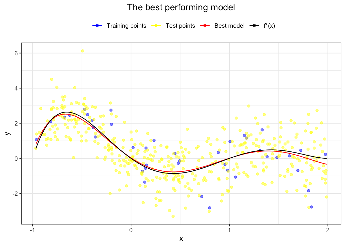

Not bad! Our model fits very well and often overlaps the “true” function $f^{\ast }$.

Note the danger of extrapolation! The regression we found fits well only within the defined region, and we have no reason to assume it will look like $f^{\ast }$ beyond it.

Training Samples

How do these errors behave when we keep increasing the training sample size? Let’s stick with the best model we found previously. We will train it on varying training sample sizes, $n=10,11,...,50$ and each time use the remaining data to find the testing error.

Then we plot the training sample size $n$ against the prediction errors for the training and testing sets. Here’s what we get:

training_n = c()
testing_n = c()

for (n in 10:50){
  train <- sample[1:n,]
  test <- na.omit(sample[n+1:450,])
  
  reg <- lm(y ~ poly(x, 5), data = train)
  pred_test <- predict(reg, test[,1])
  
  training_n[n-9] = sum((reg$residuals)^2) / n
  testing_n[n-9] = sum((test[,2] - pred_test)^2) / (450 - n)
}

obs_seq = seq(10, 50)

final_df = data.frame(cbind(obs_seq, training_n, testing_n))

ggplot(final_df, aes(obs_seq, training_n, colour = "Training")) + geom_line() +
  geom_line(aes(obs_seq, testing_n, colour = "Testing")) + theme_bw() +
  scale_colour_manual("", 
                      breaks = c("Training", "Testing"),
                      values = c("blue", "yellow")) +
  labs(title = "Prediction error against amount of training data",
       x = "Training data size (n)", y = "prediction error") +
  geom_text(x = 18, y = 1.5, label = "Big drop", inherit.aes = FALSE, colour = "red") +
  theme(plot.title = element_text(hjust=0.5), legend.position = "top")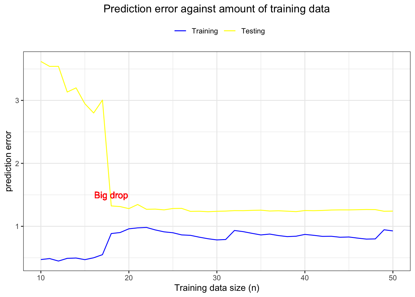

The training error increases with a bigger sample size - we are less prone to fit the noise when there is more available data. The testing error steadily decreases up to a point where it drops significantly ($n=18$ in our case), then it keeps going down but only slightly. The drop occurs fairly quickly because our model is not complicated - if it were, we would need more training points to capture the data structure. The conclusion is simple, the more data we have, the better. However, it is possible to find a data size that gives comparable prediction results as if we used more data.